Functional programming is a style of programming which place the emphasis on
functions. Functions helps to clearly express the intent of a piece of code. To
me, R is a functional language. Its deep roots goes back to Scheme, a
functional LISP dialect. The imperative part of R are to be found in its S
legacy. In this post, I want to describe how I use functions in R, mixing
imperative and purely functional programming.
I will take as an example an analysis I’ve done in the past few months. It was a quick one day long analysis, but I think it would have been much longer if I had not used R1.
I work in biology. In november, we received results of a run of Sanger sequencing. It was done in 96 well plates on 800bp PCR amplicons. We quickly found out that some sequences showed traces of contamination : we had secondary peak specifically on our divergence markers. We had reasons to believe that sequences with secondary peak would be distributed randomly over the 96 well plate if it was not a sign of contamination. I decided to test the random distribution using a quick simulation.
The simulation would do the following :
- generate 96 well plates with as much contaminated well as there were in our plates.
- generate a lot of those plates.
- per well, count the average number of contaminated well, and average this count over the plate.
- compare this simulated statistic with the observed one in our plate.
We first need to load some packages.
library(assertthat)
library(ggplot2)
library(dplyr)
Functions express intent
We want a simple function to sample a number at random between 1 and n.
random_well <- function(n) sample(1:n, 1)
This function does only one simple thing. But it has a name that clearly express what it does and abstracts the sampling process, so simple as it is.
We also want a simple function to generate an empty plate, ie a plate where no well is contaminated. A 96 well plate can easily be represented as a 8 by 12 matrix.
initiate_plate <- function() matrix(rep(0, 96), nrow = 8, ncol = 12)
In the same manner, the function is really simple, but now I can just call
initiate_plate and be done with it : I now have an 8 by 12 matrix with 0 all
over, ready to be filled up with simulated contaminations !
Recursion shortens the distance from mind to code
We now want to contaminate n well inside of this empty plate.
plate_generate <- function(plate = initiate_plate(), n) {
    assert_that(is.numeric(n), n < 96)

    ## this function contaminate a plate well if it is not already contaminated.
    ## it uses recursion to do so.
    contaminer <- function(mat) {
        x <- random_well(8) # sample one line at random
        y <- random_well(12) # sample one column at random

        if (mat[x, y] != 1) {
            mat[x, y] <- 1
            mat
        } else {
            contaminer(mat)
        }
    }

    ## if the plate already have *n* contaminated wells, return it.
    ## otherwise create a plate with *n - 1* contaminated wells.
    ## this kind of recursion is particularly useful to think about.
    if (sum(plate < n)) {
        ## if the plate does not have n wells contaminated
        contaminer(plate_generate(plate, n - 1))
        ## generate another plate with *n - 1* contaminated wells,
        ## and contaminate another random well.
    } else {
        plate
    }
}
plate_generator uses recursion. It is a style of function calling that I
believe to be discouraged in R. But as my stack cannot exceed 96, I can use
recursion without worrying too much about overflowing the R stack.
I have enclosed a function inside of it, since I do not need it outside of this
context. This function, contaminer, set the well / matrix value to 1 at a
random coordinate if the well is not already at 1. If the well is already
contaminated (equals to 1), I call contaminer on the plate again : it will
pick another random well, and contaminate it. If the well is already
contaminated (equals to 1), I call contaminer on the plate again : it will
pick another random well, and contaminate it. If the well is already … I think
you begin to understand how recursion works.
plate_generator uses contaminer to create a matrix with n contamination
inside, ie n wells with a 1 value and 96 - n wells with a 0 value. It does
so by first checking if the total count of plate is equals to n. If not, we
can generate a plate with n - 1 contamination, and add another contamination
with contaminer. How can we generate a plate with n - 1 contamination ? It
would be great if we had a function that generate a plate with the desired
amount of contamination. Well, it appears we have. This function is called
plate_generator. If we call plate_generator with n = n - 1, it will
contaminate another well ; the plate sum is now equal to n and we can return
it. But generating a plate with n - 1 contaminated well implies that we have a
plate with n - 2 contaminated well and so on. This is recursion. I have one
function that does one thing and call itself to reach its goal.
The plate_generator function is useful in the sense that I did not have to
think about it really well. I know it is not optimised. I know that I can
shorten the time of execution by first excluding wells that are already
contaminated from the parameters space of contaminer, instead of picking
/ checking / contaminating a well randomly. The function would gain in speed.
But I can generate ten thousands plate on my computer in less than 2 minutes.
The function did not take that long to develop.
The previous code is maybe a little bit tedious to understand. Anyway, once it is tested, I do not have to care about how it is done. I can just call the function, I know it will always give the same result, even if the implementation change. It is a level of abstraction that clearly helps to develop clean and clever code by iterative steps. I am not afraid of breaking everything up : I know my functions does one thing and does it well. It has no side-effects. This function is pure : it does not modify anything outside its scope.
We now want to generate many random plates, with a finite number of contamination inside of it.
Running the simulation
n_plate_generate <- function(number_of_plate, number_of_conta) {
    lapply(1:number_of_plate, function(i) plate_generate(n = number_of_conta))
}
We now can generate three plates with three contaminated wells inside of it.
n_plate_generate(3, 3)
## [[1]]
##      [,1] [,2] [,3] [,4] [,5] [,6] [,7] [,8] [,9] [,10] [,11] [,12]
## [1,]    0    0    0    0    0    0    0    0    0     0     1     0
## [2,]    0    0    0    0    0    0    0    0    0     0     0     0
## [3,]    0    0    0    0    0    0    1    0    0     0     0     0
## [4,]    0    0    0    0    0    0    0    0    0     0     0     0
## [5,]    0    0    0    0    0    0    0    0    0     0     0     0
## [6,]    1    0    0    0    0    0    0    0    0     0     0     0
## [7,]    0    0    0    0    0    0    0    0    0     0     0     0
## [8,]    0    0    0    0    0    0    0    0    0     0     0     0
##
## [[2]]
##      [,1] [,2] [,3] [,4] [,5] [,6] [,7] [,8] [,9] [,10] [,11] [,12]
## [1,]    0    0    0    0    0    0    0    0    0     0     0     0
## [2,]    0    0    0    0    0    0    0    0    0     0     0     0
## [3,]    0    0    1    0    0    0    0    0    0     0     0     0
## [4,]    0    0    0    0    0    0    0    0    0     0     0     0
## [5,]    0    1    0    0    0    0    0    0    0     0     0     0
## [6,]    0    0    0    0    0    0    0    0    0     0     0     0
## [7,]    0    0    0    0    1    0    0    0    0     0     0     0
## [8,]    0    0    0    0    0    0    0    0    0     0     0     0
##
## [[3]]
##      [,1] [,2] [,3] [,4] [,5] [,6] [,7] [,8] [,9] [,10] [,11] [,12]
## [1,]    0    0    0    0    0    0    0    0    0     0     0     0
## [2,]    0    0    0    0    0    0    0    0    0     0     0     0
## [3,]    0    0    0    0    0    0    1    0    0     0     0     0
## [4,]    0    0    0    0    0    0    0    0    0     0     0     0
## [5,]    0    0    0    0    0    0    0    0    0     0     0     0
## [6,]    0    0    0    0    0    0    0    0    0     0     0     0
## [7,]    0    0    0    0    0    0    0    0    0     0     0     0
## [8,]    0    1    0    1    0    0    0    0    0     0     0     0
We then need to count, per well, the number of neighbouring contaminated well. This function is kinda tricky to explain, and demands some kind of expertise with typical biological plates. I had to hardcode many stuff, so I guess this is not the cleaner way to do it. But at least is works.
has_nearby_conta <- function(plate, line, column) {
    assert_that(is.matrix(plate), is.numeric(line), is.numeric(column))

    x      <- line
    y      <- column
    p      <- plate
    nearby <- c()

    bord_gauche     <- function(col) ifelse(col == 1 , TRUE, FALSE)
    bord_droite     <- function(col) ifelse(col == 12, TRUE, FALSE)
    bord_sup        <- function(row) ifelse(row == 1 , TRUE, FALSE)
    bord_inf        <- function(row) ifelse(row == 8 , TRUE, FALSE)

    coin_sup_gauche <- function(row, col) ifelse(bord_gauche(col) & bord_sup(row), TRUE, FALSE)
    coin_inf_gauche <- function(row, col) ifelse(bord_gauche(col) & bord_inf(row), TRUE, FALSE)
    coin_inf_droite <- function(row, col) ifelse(bord_droite(col) & bord_inf(row), TRUE, FALSE)
    coin_sup_droite <- function(row, col) ifelse(bord_droite(col) & bord_sup(row), TRUE, FALSE)

    if      (coin_sup_gauche(x, y)) { nearby <- c(nearby, p[x, y+1], p[x+1, y+1], p[x+1, y])}
    else if (coin_inf_gauche(x, y)) { nearby <- c(nearby, p[x-1, y], p[x-1, y+1], p[x, y+1])}
    else if (coin_sup_droite(x, y)) { nearby <- c(nearby, p[x, y-1], p[x+1, y-1], p[x+1, y])}
    else if (coin_inf_droite(x, y)) { nearby <- c(nearby, p[x, y-1], p[x-1, y-1], p[x-1, y])}
    else if (bord_gauche(y))        { nearby <- c(nearby, p[x-1, y], p[x-1, y+1], p[x, y+1], p[x+1, y+1], p[x+1, y])}
    else if (bord_droite(y))        { nearby <- c(nearby, p[x-1, y], p[x-1, y-1], p[x, y-1], p[x+1, y-1], p[x+1, y])}
    else if (bord_sup(x))           { nearby <- c(nearby, p[x, y-1], p[x+1, y-1], p[x+1, y], p[x+1, y+1], p[x, y+1])}
    else if (bord_inf(x))           { nearby <- c(nearby, p[x, y-1], p[x-1, y-1], p[x-1, y], p[x-1, y+1], p[x, y+1])}
    else {
        nearby <- c(nearby,
                    p[x-1, y-1], p[x, y-1], p[x+1, y-1],
                    p[x-1, y  ],            p[x+1, y  ],
                    p[x-1, y+1], p[x, y+1], p[x+1, y+1] )
    }

    ## normalise to 1 if > 1
    nearby[nearby > 0] <- 1

    ## return the mean of the nearby matrix.
    mean(nearby)
}
We apply this function to a plate, to count the mean number of well that have at least one well contaminated.
count_nearby_conta_well <- function(plate) {
    locate_conta_well <- function(plate) {
        which(plate != 0, arr.ind = TRUE)
    }

    ## stores the positions of contaminated wells inside a list of the form
    ## ( (row . column)
    ##   (row . column) )
    well_list <- locate_conta_well(plate)

    mean(
        apply(well_list, 1,
              function(x) {
            has_nearby_conta(plate, line = x[1], column = x[2])
        }))
}
During the debugging of this function, it was particulary useful to have clean
and expressive names to decrypt the traceback() output.
We need to count the number of contaminated well inside our plate.
count_conta <- function(plate) length(which(plate != 0))
Let’s set N the number of plate in the monte carlo simulation.
n_plate <- 1000
We can then generate 1000 plates with C contamination inside of it, randomly distributed on the plate.
# generate `n_plate` with C contaminated well
random_weak <- n_plate_generate(n_plate, 35)
## count the average number of nearby contaminated well per well and average it
## over the plate. Do it to all the plate in random_weak.
random_weak_mean_list <- lapply(random_weak, count_nearby_conta_well)
Just so that you can see the data :
head(random_weak, n = 3)
## [[1]]
##      [,1] [,2] [,3] [,4] [,5] [,6] [,7] [,8] [,9] [,10] [,11] [,12]
## [1,]    1    1    0    0    0    1    1    1    0     0     0     0
## [2,]    1    0    1    0    1    1    0    1    0     0     1     0
## [3,]    0    0    0    0    0    1    1    1    1     0     0     1
## [4,]    1    1    0    0    0    0    0    0    1     0     0     0
## [5,]    1    0    0    1    0    1    1    0    1     0     0     0
## [6,]    0    0    1    0    0    1    0    0    0     0     1     1
## [7,]    0    0    0    0    0    1    0    1    0     0     1     0
## [8,]    0    1    0    1    1    0    0    0    1     0     0     0
##
## [[2]]
##      [,1] [,2] [,3] [,4] [,5] [,6] [,7] [,8] [,9] [,10] [,11] [,12]
## [1,]    1    0    0    0    0    0    1    1    1     0     1     0
## [2,]    1    0    0    0    0    1    0    0    0     0     1     1
## [3,]    0    1    1    0    0    0    0    1    0     1     0     1
## [4,]    0    1    1    0    0    0    1    0    0     0     1     0
## [5,]    0    1    0    0    1    1    0    1    0     1     1     0
## [6,]    0    1    1    0    1    0    0    0    0     0     0     0
## [7,]    0    0    0    0    1    1    1    1    0     1     0     1
## [8,]    1    0    0    0    0    0    0    0    0     1     0     0
##
## [[3]]
##      [,1] [,2] [,3] [,4] [,5] [,6] [,7] [,8] [,9] [,10] [,11] [,12]
## [1,]    0    0    0    1    1    0    0    0    0     0     0     1
## [2,]    0    0    1    0    1    1    1    0    0     1     0     1
## [3,]    0    1    0    0    1    0    0    0    0     1     1     1
## [4,]    0    0    0    0    1    1    0    1    0     1     1     0
## [5,]    1    0    0    0    1    0    0    0    1     0     0     0
## [6,]    0    0    0    1    0    0    0    1    0     0     0     1
## [7,]    0    0    0    0    1    0    0    1    0     0     1     0
## [8,]    1    1    1    0    1    1    0    0    1     0     1     0
head(random_weak_mean_list, n = 3)
## [[1]]
## [1] 0.3440476
##
## [[2]]
## [1] 0.3188095
##
## [[3]]
## [1] 0.3590476
For the first plate, the 96 wells have a mean of 0.3440476 wells contaminated.
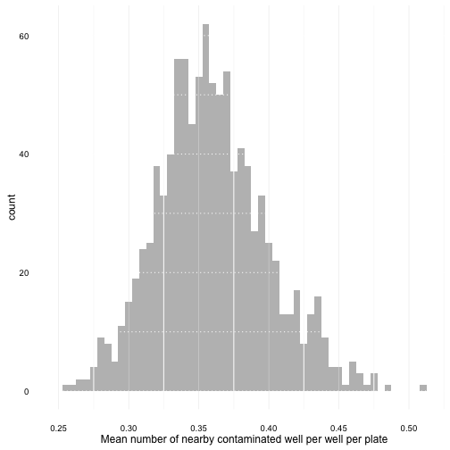
plot_mean_distrib <- function(random_mean_list) {

    random_mean_list %>%
        unlist() %>%
        data.frame(wellcount = .) %>%
        ggplot(aes(wellcount)) +
        geom_histogram(binwidth = 0.005, fill = "gray") +
        labs(x = "Mean number of nearby contaminated well per well per plate") +
        theme_minimal() +
        theme(panel.ontop = TRUE,
              panel.grid.major.y =
                  element_line(colour = "white", size = 0.5, linetype = "dotted"),
              panel.grid.minor.y =
                  element_line(colour = "white", size = 0.5, linetype = "dotted"))

}
A first plot :
plot_mean_distrib(random_weak_mean_list)
Factorial in R :
I think this function is the cleanest and fastest way to express the factorial
function in R. And yes, * is a function.
factorial <- function(n) {
    Reduce(f = `*`, x = 1:n, init = 1)
}
- Actually it is the language I am the most comfortable with, so it is not really a good comparison… [return]